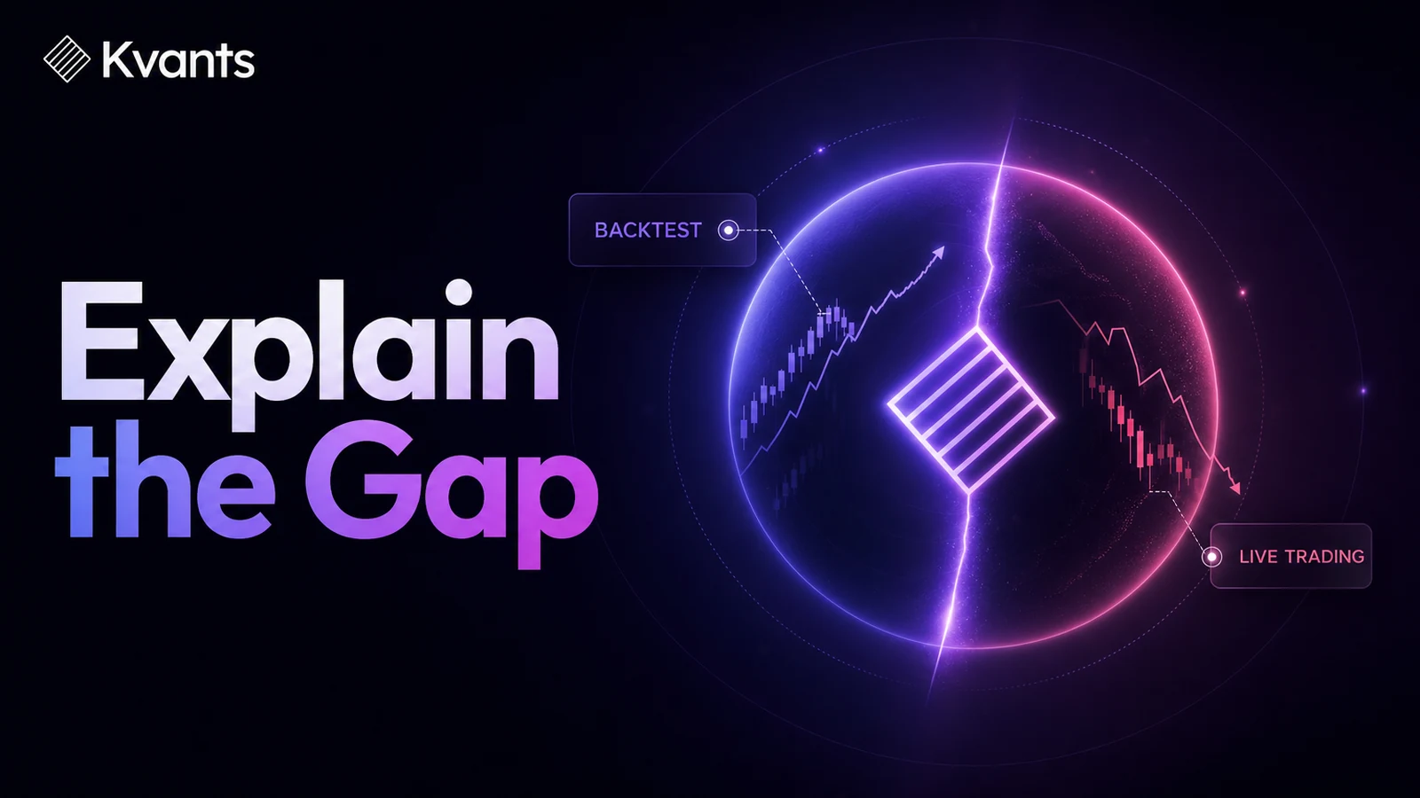
Learn why backtest and live trading results diverge, how to diagnose the performance gap, and when execution problems—not strategy failure—are the likely cause.
Quick Answer
Backtest and live trading results differ because a backtest is a model, while live trading includes uncertain fills, changing liquidity, operational delays, and human decisions. A gap does not automatically mean the strategy has failed. First compare identical rules, costs, position sizing, and eligible signals. Then separate the difference into simulation error, execution error, sampling variation, and market-regime change. The main limitation is that a short live record rarely contains enough trades to identify the cause with confidence.
Key Takeaways
- A backtest estimates how rules would have behaved under specific data and execution assumptions; it does not predict exact live results.
- Compare normalized returns, such as R multiples, rather than raw dollars when position size has changed.
- Audit missed, added, delayed, and incorrectly sized trades before concluding that the underlying strategy deteriorated.
- Slippage, spread, fees, and order sequencing can erase a small historical edge.
- Live results need an adequate sample and comparable market conditions before they can challenge the backtest.
- Use paper and limited-risk deployment as diagnostic stages, not as proof that future performance is assured.
Backtest vs Live Trading: What Each One Measures
A backtest applies defined trading rules to historical market data. Its output depends on the available data, the strategy logic, and assumptions about order activation, fills, costs, and position sizing.
Live trading submits orders into an unfolding market. Prices can move while an order is in transit. Available liquidity can vary, stops can fill beyond their trigger prices, and discretionary decisions can alter the intended rules.
Neither method is a universal winner. They answer different questions.
| Method | Best For | Main Limitation | Evidence Produced |
|---|---|---|---|
| Backtesting | Evaluating rules across many historical trades and market conditions | Results depend on data quality and simulation assumptions | A conditional estimate of historical strategy behavior |
| Paper trading | Checking signals, order handling, and workflow without risking capital | Simulated fills and behavior may still differ from live execution | Evidence that the strategy can be operated prospectively |
| Live trading | Measuring realized fills, costs, operational reliability, and rule adherence | Capital is at risk, and samples accumulate slowly | Actual execution results under the observed conditions |
The useful comparison is therefore not “Which method is accurate?” It is “Which source of uncertainty does each stage expose?”
A backtest's equity curve and trade-by-trade log.
The Four Sources of the Performance Gap
1. Simulation assumptions
A backtest must decide when an order becomes active and what price it receives. Problems arise when those assumptions are more favorable than real execution.
Common examples include:
- Filling a market order at the signal candle’s close even though the signal was not known until that close
- Assuming every limit order fills when price merely touches the limit
- Ignoring spread, commissions, funding, or other trading costs
- Filling a stop at its trigger price during a fast move
- Resolving a same-bar stop and target in the favorable order without lower-timeframe evidence
These errors are most damaging when the strategy targets small moves. A cost or fill difference of 0.05R may be modest for one trade but decisive across a strategy with thin expectancy.
2. Execution differences
Even a realistic backtest cannot ensure that the live strategy follows the same specification. The live implementation may calculate an indicator differently, evaluate signals at another time, or use a different order type.
Create an execution reconciliation log with four categories:
- Matched: the backtest and live process both took the trade.
- Missed: the historical rules qualified, but no live trade was taken.
- Added: a live trade was taken even though the tested rules did not qualify.
- Mismatched: both took the trade, but the entry, exit, size, or timing differed.
This trade-level comparison is more informative than looking only at total profit and loss.
3. Sampling variation
A strategy with positive historical expectancy can produce a losing live sequence. Win rate, average winner, and drawdown vary from one sample to another.
Suppose a strategy produced 500 historical trades but has only 18 live trades. The live win rate can differ sharply without providing strong evidence of structural failure. The question is not whether the two percentages are identical. It is whether the live outcome remains plausible given the range of historical sequences and current execution quality.
Review rolling windows and the distribution of losing streaks rather than comparing one full backtest average with one small live sample.
4. Market-regime change
The live market may not resemble the conditions that dominated the backtest. Volatility, trend persistence, spreads, liquidity, correlations, and event frequency can all change.
Segment the historical record using variables relevant to the strategy. A breakout system might be grouped by volatility and trend regime. A mean-reversion strategy might be grouped by range width, session, or distance from a reference price.
If live conditions fall within a historically weak segment, the discrepancy may be regime sensitivity rather than faulty implementation. That still requires action, but it is a different diagnosis.
A strategy laid out end to end in the Kvants editor.
A Step-by-Step Diagnostic Workflow
Step 1: Freeze the strategy specification
Record the exact entry, exit, sizing, timing, and eligibility rules used in the original backtest. Do not optimize the rules while diagnosing the gap. Changing them destroys the baseline needed for comparison.
Include indicator settings, data timeframe, session boundaries, order types, cost assumptions, and handling of missing data.
Step 2: Reproduce live signals from stored data
Run the frozen strategy over the same dates covered by the live record. This creates a like-for-like comparison instead of contrasting current live trades with a long historical average.
Confirm that the research process and live workflow generated the same eligible signals. If not, investigate data feeds, timestamps, indicator initialization, and rule interpretation.
Step 3: Reconcile every trade
Classify each signal as matched, missed, added, or mismatched. For matched trades, compare:
- Intended entry and actual fill
- Intended stop and actual stop
- Planned size and executed size
- Modeled costs and realized costs
- Expected exit reason and actual exit reason
Express differences in R, where 1R is the planned risk on the trade. This makes comparisons more meaningful when account value or position size changes.
Step 4: Recalculate with realized costs
Replace the backtest’s assumed fees, spread, and slippage with observed live values where possible. Use distributions rather than one optimistic average if costs vary materially by volatility or time of day.
If the adjusted backtest approaches the live outcome, the problem is likely execution economics rather than the entry signal itself.
Step 5: Compare equivalent conditions
Filter historical trades to conditions resembling the live period. Compare the same instruments, sessions, volatility range, direction, and strategy version.
This analysis should have been defined in advance where possible. Searching through many filters after losses can produce a convenient but unreliable explanation.
Step 6: Choose a controlled response
The diagnosis should determine the response:
- Simulation problem: correct the backtest and reassess the strategy.
- Implementation problem: repair the logic or data pipeline before resuming.
- Rule-adherence problem: reduce discretion and strengthen the execution checklist.
- Cost problem: revise order handling or reject strategies whose edge is too small after costs.
- Possible regime change: reduce exposure, gather more evidence, and apply predefined pause criteria.
Avoid rewriting the strategy solely to explain a short losing sequence.
Browsing tradeable signals in the research library.
Worked Example: Decomposing a Live Shortfall
Consider a hypothetical strategy with 200 backtested trades. Its gross win rate is 46%, its average winner is 1.6R, and its average loser is 1R.
Gross expectancy is:
(0.46 × 1.6R) − (0.54 × 1R) = 0.196R per trade
After modeled costs of 0.05R per trade, estimated net expectancy is 0.146R.
The first 40 live trades show a 43% win rate, an average winner of 1.45R, an average loser of 1.08R, and costs of 0.08R. Estimated live expectancy is:
(0.43 × 1.45R) − (0.57 × 1.08R) − 0.08R ≈ −0.07R per trade
The total gap is not explained by win rate alone. Winners are smaller, losses are larger, and costs are higher. The next review should inspect why exits changed, whether stops slipped, and whether discretionary trade management reduced winners.
Forty trades may still be too few to declare the strategy invalid. However, the execution differences are actionable immediately because they do not depend on proving statistical decay.
Failure Modes That Produce False Conclusions
Comparing different strategy versions
If the live rules include filters or exits absent from the backtest, the two result sets do not represent the same strategy. Version every material rule change and evaluate it separately.
Treating all divergence as psychology
Behavior matters, but blaming discipline before checking timestamps, fills, and code can hide implementation defects. Audit objective differences first.
Ignoring trades that were never taken
A journal containing only executed trades cannot show missed signals. Maintain a prospective signal log so valid but unexecuted opportunities remain visible.
Optimizing after every drawdown
Frequent adjustment fits the strategy to recent noise. Define review intervals and intervention thresholds before live deployment.
Using raw profit as the only comparison
Dollar returns are distorted by changing size and account value. Compare R multiples, trade counts, exposure, costs, and rule adherence alongside net results.
Applying the Workflow in Kvants Studio
After the diagnostic framework is defined, Kvants Studio can help translate a plain-English trading idea into editable, auditable strategy logic. Keeping the logic explicit makes it easier to verify whether the tested and deployed versions use the same conditions.
Backtests run on NautilusTrader’s event-driven engine, which supports research where order sequencing and execution assumptions matter. Parameter sweeps, walk-forward analysis, and crisis-stress validation can be used to examine whether results depend on a narrow configuration or historical period.
A strategy can then move through controlled paper and live workflows rather than jumping directly from historical results to full exposure. Pine Script v6 export is also available when TradingView is part of the workflow. The Kvants documentation explains strategy logic and export workflows, while the Kvants blog covers broader validation and risk concepts.
These tools can make assumptions easier to inspect, but they cannot eliminate market uncertainty or guarantee that historical relationships will persist.
Frequently Asked Questions
How close should live results be to a backtest?
There is no universal acceptable gap. Compare trade frequency, normalized expectancy, costs, drawdown, and rule adherence over equivalent conditions. Live outcomes should be evaluated against a plausible historical range, not one average value.
Does worse live performance mean a strategy is overfit?
Not necessarily. Overfitting is one possible cause, but unrealistic fills, higher costs, implementation errors, discretionary changes, small samples, and regime shifts can produce the same symptom. Diagnose those causes separately.
How many live trades are needed before comparing results?
The required sample depends on trade frequency and the variability of outcomes. A fixed trade count cannot guarantee confidence. Use the historical distribution of rolling samples to judge how unusual the live sequence is, and continue checking execution from the first trade.
Should paper trading match backtest results exactly?
No. Paper trading uses prospective signals and may model fills differently. Its main purpose is to test whether the strategy can be operated consistently and whether signals, orders, and records behave as intended.
When should a live strategy be paused?
Pause criteria should be defined before deployment. Examples include a breached risk limit, repeated implementation errors, costs beyond tested assumptions, or drawdown outside a predefined tolerance. A pause should trigger diagnosis, not automatic optimization.
Risk Note
This article is educational and is not investment advice. Trading involves risk, including the possible loss of capital. Backtested performance does not guarantee future results, and simulated fills may differ materially from live execution. Kvants is a research tool, not an investment adviser.